Improving Images by Fighting Noise
Imaging sensors are like the swimming pool at the country club. Not everybody is guaranteed an opportunity to swim; some photons lack membership cards. But for the most part, a typical photon would quite likely stand a good chance of swimming somewhere on the chip. Now, where I choose to swim doesn't matter so much as does the fact that I actually have opportunity to swim for a good long while, or at least until somebody drains the pool. Perhaps 35% of my h-alpha buddies don't get that chance, so call me fortunate.
Thankfully, the CCD or CMOS pool is chlorinated (or calibrated) to produce a very clean and clear swimming experience, or at least that is true until on a summer weekend when half the universe targets our pool. Let's talk about the mess that comes with that! Extra chlorine helps, but it seems that we always bring our own filth with us. I can somewhat live with that - we are what we are.
But what I can't tolerate is when the pool isn't clean before we jump in - or when the heat comes and people don't shower before swimming. Or when half-way through the day, they pull us out of the pool for a 10 minute "safety-break" head count. Talk about wasted efficiency! I guess one such count-off is okay, but every hour, on the hour? Come on!
If I really were a photon, perhaps I'd be okay with such noise. Perhaps not. But as long as management lets my voice be heard, I'd keep swimming!
________________________
Analogies aside, it seems like we deal with a lot of filthy noise in CCD/CMOS imaging. We do have strategies for mitigation in these areas - which both complicates the hobby greatly AND provides obfuscation where a deeper understanding of sensor theory is concerned. And it is this aspect of confusion that leads us to look for "rules of thumb" and truisms in the hobby. These are typically useful and safe - until they are misconstrued or wrongly-applied. For the astrophotographer, it leads us to believe that we MUST do certain things with regard to noise...or we must purchase gear based on such concerns.
But what if I told you that very little of what concerns most astrophotographers concerning noise actually affects my images? No, there are no special rules for yours truly. Nor did I stay at a Holiday Inn Express last night. Neither do I have equipment that is necessarily better than yours. Well, maybe I do, but that doesn't matter for what we will be talking about here.
Rather, you too can experience some of the same comforts, knowing that your image data represents the theoretical max in terms of noise on any given night. What if I told you that with the right imaging plan and a proper mitigation strategy that you can essentially take images with what might be close to the "ideal" camera. In fact, did you know that you actually have control over most of these things?
I know that this isn't what you've always heard. Every book and article you have read have talked about sources of noise (plural) and that it will ruin your images if you aren't careful.
As such, in this article, we will be exploring ways to yield images where the ONLY real source of noise in your images is that which you cannot control anyway, that being "photon-noise" or "object-noise." Consequently, you can maximize the efficiency of your imaging by assuring yourself the highest signal-noise ratio possible by producing images with the lowest amount of NOISE possible. (NOTE: To see what this looks like from the standpoint of improving SIGNAL, see my article, "Best Data Acquisition Practices" here.)
Therefore, this article looks at how the astrophotographer can develop a plan for achieving optimal images from the standpoint of "noise" with their cameras.
|
HOW NOISE ACCUMULATES IN AN IMAGE...
Toward that end, let's first examine how noise in an image could potentially interact, to establish WHY we need techniques and strategies to handle it. Astrophotographers have come to understand the total unpredictability in a region of pixels - you need more than one pixel to measure it - as noise, even if they may not fully understand the mechanisms that produce it or the scale in which it shows itself. Mistakenly, from the classical thought of "noise" from other fields (like television and music), noise is NOT "unwanted signal." Unwanted signal is an important subject of its own and requires its own section (it's actually more important of a discussion from the standpoint of practicality). But when we regard noise as "variance from expected values," as we should, we will be dealing with MANY sources of noise, all of which we will talk about here in due time. But the one thing that every imager should understand FIRST is that these noise sources (within an image) always add quadratically. For all sources of noise, the total amount of noise would be represented by the square root of the sums of their squares. As such... total noise = sqrt (source 1^2 + source 2^2 + ... + source n^2) When this is properly understood, then the imager can work to reduce the total effect of noise in an image if they can minimize the contributions of noise sources compared to others. Many sources of such noise can be calibrated out of the image. Others, can be diminished through a good mitigation strategy. For example (and as a tease to what follows in the article), a high read-noise camera at 15 e- doesn't have to impact an image much if I can "swamp it" within another source of noise, as follows... Total noise = sqrt (100 e- shot noise ^2 + 15 e- read noise ^2) = 101.1 e- You've undoubtedly heard that camera read noise is "bad," but in such a case, it contributes only 1% of the overall amount of noise in the sampled area, assuming these are the only two noise sources in this hypothetical example. There is a revelation hidden in those numbers somewhere and later we might find it. But for now, if you understand the concept of hiding smaller noise sources within larger sources, especially within a single, dominant source of noise that we cannot control anyway, then you have an idea of what we will seek to do here, which is to image with a camera we didn't even know we had...a near perfect one. NOISE SOURCES Let's sort types of noise within two-broad categories, random noise and spatial noise. You will see that we can do nothing about random noise, other than do our best to mitigate those sources, which I will show you how to do later. These sources end up in the image and accumulate according to the equation I showed earlier. These sources include shot (Poisson) noise (from the object and the sky-background) and camera read noise. On the other hand, spatial noise is related to a pattern, which can be modeled and mostly (not completely) removed through calibration techniques. We will see that there is spatial noise relating to pixel gain (how an amplifier boosts signal) and that relating to offset (how an amplifier is reset). There is another category of "noise" which you think is noise but really isn't noise. This is unwanted signal, which people confuse as noise. This will be handled in its own section. NOTE: The problem with an amateur astronomer trying to understand noise is that NOBODY can agree on what to call the various sources. Be patient and I talk about the sources within a more understandable context, where I will try to clarify all of the jargon, along with the cause of these sources. Random Noise Sources The problem with "random" is that you cannot do anything about it. However, with longer total imaging time (increased signal), the randomness can be averaged out. Likewise, an understanding of this will help you better understand why stacking multiple images can help diminish this category of noise. So, let's first take a look at the type of noise that will become our main contributor to our images... 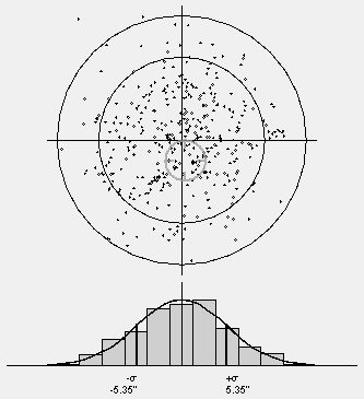
FIgure 1 - When a shotgun is fired, it scatters pellets in a natural distribution as shown. A histogram can show the distribution from the center of the target. The first ring represents the standard deviation (1st sigma) of the distribution of pellets, which in this case is at +/- 5.35" from the center. In any standard distribution, like this, approximately 68% of all pellets will be inside the first ring...a value which becomes more predictable at higher numbers of pellets. In astronomy, the image sensor records photons exactly the same way, creating the star profiles we see, despite the fact that they are coming from a "point source." Thus, light is scattered very predictably, despite randomly hitting the target.
- Credit www.shotgun-Insight.com
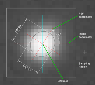 A star's profile is measured by the FWHM (the width of the diameter of a star at half its maximum pixel value). Compared to a normal distribution, this width occurs after the standard deviation. In fact, it takes 2.335 sigmas to equal the star's width at its half-maximum. This means that approximately 80% of the photons of a star will be contained within its FWHM. A star's profile is measured by the FWHM (the width of the diameter of a star at half its maximum pixel value). Compared to a normal distribution, this width occurs after the standard deviation. In fact, it takes 2.335 sigmas to equal the star's width at its half-maximum. This means that approximately 80% of the photons of a star will be contained within its FWHM.
Shot or Photon Noise
Shot Noise or Photon noise, also known as "Poisson" noise, is the noise arising from the natural distribution of random events. It is the unavoidable result of collecting millions of photons on an imaging chip, each of which is a single, random event. Like a shotgun which randomly scatters the contents of its shell over some area, light from space does the same onto your imaging sensor (see FIGURE 1 above). But while I cannot predict exactly where photons will fall, I CAN make a judgment about how they will be distributed across a group of pixels. The most obvious way to see this happening in astronomy is by looking at a star in your image, which might represent a million total photons hitting your chip. Though a point source of light, one might expect the star energy to show up on one and only one pixel. Instead, star energy distributes strongly in the center, tapering off to the edges, spanning multiple pixels. A star's point-spread function (PSF) or star profile would show ~68% of the star light concentrated within 1 standard deviation (or sigma) of the center, 95% within 2 sigma, and 99% within 3 sigma. This can be witnessed in the illustration above. Keep in mind, once again, that in a perfect universe light coming from a single point source SHOULD end up in one pixel only. But the normal distribution demands otherwise. For stars, we really don't mind such imperfection, since the resulting image seems to contain real looking stars. However, what is probably not that apparent to you in the illustration is that the pixels you might think have the same values actually don't. For example, in the pixels marking the FWHM (full-width, half-maximum) of the star above (see the ellipse shape), you might think that those pixels would have the same value, being more or less equidistant from the star's center...but truly they do not. They vary ever so slightly. This is because a normal distribution of random events only TRENDS toward being more and more certain with greater numbers of events (more photons in our context). There is still variance in the distribution, meaning that if neighboring pixels have the same value, then it is a chance occurrence only. As such, at the pixel level, the amount of shot noise can be estimated as the square root of the signal. As a simplistic (and somewhat flawed) example, if 10,000 photons SHOULD be recorded at a pixel, then the actual recorded count could be within plus/minus the sqrt (10,000) or +/- 100 photons. Such a pixel would therefore contain between 9,900 and 10,100 actual electron counts (e-), which typically show in your data acquisition software as ADUs (analog-to-digital units). Interestingly, the variance (or noise) isn't really detectible in the bright areas of an image (where the bright pixels are). This is because the signal so outweighs the noise in those high SNR areas. |
Sidebar: Why is Noise So Annoying?Several factors determine how bothersome noise is within an image. They include...
Because of this, your NEED to mitigate noise will depend, in part, in how you wish to view your final image or how sensitive you are to it. For example, Noise can be seen as the obfuscation of structure. This could be the breaking up of the lines of a nebular wall, the inability to see the dimensions of a dust cloud you KNOW is there, or the surprise mottling of color that breaks up an otherwise single-hued space. As such, random noise is more visible (and objectionable) when it is "spatially-correlated," which is a fancy way of saying that noise is best perceived within a broader context of details in an image. Random noise in random space (spatially-uncorrelated) isn't as bothersome. Mouse-over the image below... 
The original image represents a gradient using shades of gray ranging from 1 bit (2^1) to 8-bits (2^8). Until we get to the 8-bit gradient (256 individual shades), the borders between shades are easily seen.
Upon mouseover, the new image shown has been injected with random (Gaussian) noise. There are some important points to be gained in this exercise. First, notice that noise is most hidden in the brighter areas (where only dark pixel noise is obvious). Similarly, neighboring high contrast areas are the least obstructed, since it remains clear where one region starts and another stops. In other words, a large amount of difference (high contrast) between neighboring shades will survive the impact of the noise from the standpoint of "detectability." So, if you hope to see details in the shadow area of an image (which have lower SNR and very little separation of values to begin with), then you have to do a lot of things right in terms of both signal acquisition and noise mitigation. Secondly, notice how the noise almost completely washes away the divisions of the 4-bit image. In practical terms, this means your high dynamic range camera will actually be limited by the noise inherent in the image, not the camera's own bit rate. This is demonstrated above in the sense that a camera capable of 8-bits of range (256 shades) is turned into a 3-bit camera (8 shades) by the amount of noise in the image. In real astrophotography terms, even though your camera might use a 14-bit analog-digital converter (ADC) to digitize your image, noise typically reduces the dynamic range to something closer to 10-bits of information in a best-case outcome. Moreover, when imaging faint details, more data will be needed to yield enough dynamic range to combat whatever noise is attempting to conceal it. This explains why people put hours upon hours of time into their images in an effort to get smooth backgrounds. Most importantly for our understanding here is that noise disguises smaller features before the larger ones. Once again, mouse-over the following image: 
As in the first example, random noise is injected to the image upon mouse-over. The varying sized polka-dots become mostly obscured by the noise with the exception of the largest of the dots. Smaller features are completely undetectable here...and if the original image wasn't posted first, you would likely not realize how many smaller dots there were. It's the last sentence that is the key takeaway here...smaller structures can hide within multiple, noisy pixels covering an area, so much so that they go beyond detection.
Now consider an image like the Hubble Deep Space field, with noise injected in much the same way. I think we begin to realize that such tiny galaxies would disappear if hours upon days of exposure time is not done. How noise affects the varying scales of an image plays a large role into how we post-process our images with noise reduction techniques. If larger details in an image are less affected by noise, then techniques that reduce noise aggressively at a small scale will be beneficial. As such, an image processing program like PixInsight will provide opportunity to customize noise reduction based upon the scale of structure that is most affected by noise, which powerfully addresses the issue without compromising image areas that do not require it. In other words, while being more difficult to learn, such software processes can allow the user to determine how aggressive they want to be with noise reduction on the areas they need it, no longer being forced to apply such tasks globally within areas that do not need it. Now, look at the same images side-by-side (below), but this time at a smaller scale. We know that the noise in the second image exists, but when viewed here, it becomes difficult to know which image is the more noisy image. The uninitiated might think that the images are the same, only the one of the right uses gray ink instead of black? This demonstrates that noise might not be perceived at all, even when you know that noise exists. Thus, noise in an image is about perception. It's about interpretation. It's about context and our satisfaction with how we see details within that context. Noise keeps us from seeing details clearly in areas we want to see - which is why we might choose to keep our backgrounds a little on the dark side of things or present our images on Facebook in smaller sizes - and it lessens dynamic range, which equates a dimensioning of the "palette" of available shades (or colors) to represent details within our image. Finally, noise itself might not be random at all, but rather conform to some sort of pattern. This is typical of various camera effects, collectively known as Fixed Pattern Noise (FPN). We perceive patterns strongly in nature, so when noise takes such a shape, especially in vertical and horizontal lines, then the effects of the noise is much worse than if the same amount of noise fell on random pixels. Thankfully, we can remove most such sources from an image through calibration techniques. "But if you understand the concept of hiding smaller noise sources within larger sources, especially within a single, dominant source of noise that we cannot control anyway, then you have an idea of what we will seek to do here, which is to approach the performance of the theoretical, perfect camera where all sources of traditional camera noise are greatly diminished. " |
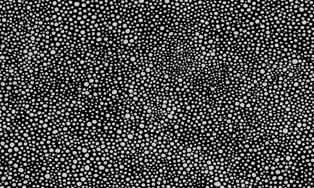

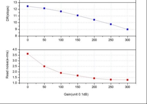 FIGURE 3 - One of the most popular, reasonably priced cameras in use today is the ZWO ASI 1600mm CMOS camera. Learning to read a camera's sensor charts can be very helpful. Here, we see the trade-off for increasing the gain of the sensor, namely, that we gain an advantage in terms of read noise performance (graph #2) at the penalty of losing dynamic range (graph #1). Understanding this trade-off in light of your imaging goal is important, which could be the subject of its own article.
But what about those areas that receive very little signal to begin with? Notice in the core of the star that noise is hardly perceived, but when you look at the background, you begin to see the characteristic salt-and-pepper look of noise from pixel to pixel. The reason is that our concept of a "smooth" image does not comes from the bright areas of an image, but rather in the dark shadow areas, where there exists less object signal as compared to the noise. In other words, it's not so much the noise we perceive, but rather the lack of quality signal necessary in the area of detail being viewed.
What's not immediately realized is that shot noise is also responsible for remnant noise from other "signal" sources, such as dark current and background light pollution (see the section on Unwanted Signal). Even upon sensor calibration and LP gradient removal, this residue persists as a noise variance. When we talk about this later, you will realize how large a concern this truly is!
But from the standpoint of shot noise, regardless of photon source, our goal becomes raising the SNR of areas of an image where we desire to show the faintest details in the objects we care about. Typically, this is done through longer TOTAL exposure times, but when you understand the dynamics of an overall system, you begin to realize that you can also accomplish this by imaging more efficiently (et al. more stable seeing; darker skies; better focus, tracking, and autoguiding; optimizing sub-exposure lengths).
Camera Read Noise
Every camera has electronics to count off the charges that are now collected within the pixels. These charges are amplified and sent to an Analog-to-Digital Converter (ADC) to be counted and stored as digital information.
The issue with amplifiers, whether in a CCD or in a hi-fi stereo system, is that they generate random noise in their use. With a camera, this occurs EVERY time you read-off the chip; with each shot you take. Consequently, a certain amount of noise gets added into the values of each pixel.
In addition, there are secondary components to camera read noise that camera manufacturers might roll into this category of random noise, including "reset" noise, or variance in how the pixels are cleared or "reset" for the next exposure (there will always be some residual charges and different manufacturers have different ways of rating their cameras in terms of read noise to reflect this).
Speaking of which, cameras will be rated according to the RMS (root-mean-square) value of pixel groups, usually something like 10e- RMS. For you, it simply means that if you look at a group of pixels in an image, there could be plus/minus 10 ADU values of difference between all the pixels upon readout of the sensor. Call it the cost of doing business...as much as we would like all pixels to be the same, they never will be.
Trying to distinguish "good" from "bad" when it comes to a "clean" camera from this standpoint is a difficult task, but there are generally 5 aspects of camera read noise you should understand, both in camera choice and overall performance.
1.) The more pixels being read-off, the more read noise you will have. As such, binning the sensor (in some cases) can improve actual read noise performance.
2.) The higher the gain of the camera, the less read noise there will be (at a cost of dynamic range). As such, there is a trade-off for camera sensors with user-adjustable gain (see FIGURE 3 at right).
3.) Read noise is spatially related, meaning that higher values from sensor to sensor are meaningless unless the pixel size is also considered. For example, a 3 e- read noise sensor with 5 micron pixels will yield similar SNR as a 12 e- read noise sensor with 10 micron pixels. Don't immediately discount a CCD chip because of the shiny new "low-read noise" CMOS chip. The pixel sizes might make them behave somewhat equally.
4.) Higher read-noise requires longer sub-exposures to lessen its impact, but it doesn't necessarily make the camera a "worse" camera. We will hit this point hard and heavy later in the article, but for now you should know that a good mitigation strategy can make even high-read noise cameras work well for you.
5.) The more sub-exposures you have, the more instances of read-noise there are to impact the image, so all else being equal, limiting the total number of sub-exposures lessens the impact.
Most of the mitigation strategies within this article concern itself primarily with overcoming read-noise, which dominates shorter exposures, and eliminating unwanted signal sources. In fact, our main formula for determining useful sub-exposure lengths only cares about read noise. This is because the other noise sources we will talk about next will be addressed though image "calibration" to render their overall impact to insignificant levels. Camera read noise is immune to this, unfortunately.
Spatial "Noise" Sources*
The total number of potential charges in a pixel is what we refer to the "well-depth" of a sensor, whereas the saturation of a pixel would be called the "full-well capacity" (FWC). Since a photon frees an electron charge in the silicon, the collection of these charges in a pixel becomes a voltage. After amplification, these voltage levels are digitized, becoming our "counts," our DNs (digital numbers), or our ADUs (analog-digital units)...whatever term you have come to use. This is a fundamental and immutable aspect to sensor technology. Some specifics to aid future understanding, particularly in how noise can be oriented in spatial "patterns"...
Transistors store the voltage within a pixel and the capacity of these transistors determines the well-depth. But such components will not always have the same exact capacities, nor will they have the same "zero" state. You can imagine how difficult it might be to make millions of transistors in a sensor all work uniformly, each of which stores these voltages in, perhaps, thousandths of a volt.
Thus, in the same way an oscilloscope or voltmeter (multi-meter) might have a margin of error when measuring the voltage of some generic circuit, there is always a margin of error from pixel to pixel. Just because something can be measured in a "thousandths" doesn't mean it's necessarily precise. You can also imagine what it's like to assure there are zero charges in these "wells" once a new exposure begins. Some residual will likely remain. Also, because these voltages have to be "clocked" off the chips and counted, there is error that arises in the transport of those charges to the ADC...and as a general rule, the faster the read-out rate (their clock frequency), the more noise there will be.
As such, these imprecisions are what is responsible for camera read-noise. These pixel errors are unpredictable, changing each time the camera is read-out. This, by definition, is true noise, or variance away from values we can predict.
Somewhat conversely, because transistors must be "biased" in order for electrical current to move through them, a voltage will always be present to permit operation (there is no true zero voltage where transistors are concerned). This bias voltage, however, is a value known for each pixel - the bias voltages do vary slightly - and can be accounted for. Astrophotographers can see this modeled well when taking a "bias frame." You can see this "pattern" behavior clearly when several bias frames are averaged together (see FIGURE below). But do not confuse this with "noise," as this is a predictable "offset" for each pixel and can be easily subtracted later when performing your data calibration.
As such, spatial noise has both gain (how signal is amplified) and offset (how amplifiers are biased) components. When we add a time component (exposure length), these noise sources will begin to rise.
Types of Pattern Noise and Its Sources
Another way a pixel varies is in how charges are accumulated over time, according to the nature of how silicon works in the chemical conversion of photons to electron charges AND how other components on the sensor add extra charges to many or all of the pixel wells, once again something that occurs over time.
ASIDE: If you wonder why your CCD camera is no longer as sensitive as it one was, consider that the ability of silicon to give up an electron when charged by a photon is based on chemistry. Not only that, the ability of transistors to move charges around is ALSO based on a chemical process called "doping" - electrons move around between positive (boron or "p-doped") silicon and negative (phosphorus or "n-doped") silicon regions (study how a diode works for the simplest explanation for electron movement in a circuit). Since there is no such thing as "free energy" and because the chemical "fuel" dissipates over time, sensors change physically over their life-spans. With heavy use, if should not be a surprise when your 10 year old CCD camera doesn't seem to work as well as it once did.
While the overall sensor can be rated according to how well it records photons over time by spectra - different wave lengths are recorded with different sensitivities - each individual pixel will be slightly different from this average measure, or something known as Quantum Efficiency. Simplified as "QE," quantum efficiency could be considered a measure of the "success rate" in which a sensor converts photons to electron charges. Truly, you should know that NOT every photon that hits the sensor is recorded...in most cases, not even by a half.
Sensor design largely determines the overall success rate, or QE, for the sensor, which we can somewhat think of as the overall sensitivity of a chip. Factors such as the existence of micro-lenses, front vs. back illumination structures, CCD vs. CMOS architectures ultimately determine how fast a camera will collect our data. In fact, it's a good idea to consider QE heavily in your next camera purchase. See SIDEBAR: KAF-16803 vs. IMX-455 for more.
Your first implication is that the varying sensitivities among the pixels will make for differing amounts of counts within the pixel wells, even if all other photon collection efforts were treated equally (remember shot noise). At fewer levels of photons, either in lower light levels or in shorter amounts of time, the variance between pixels is not very perceptible, as other dominant noise sources will greatly overwhelm regions of the image. However, as the pixels reach saturation, the difference in pixel collection rates greatly impacts photon counts, to the point where the variance becomes greater than even shot noise from the sky background.
Sidebar: The Unique Fingerprint of PRNU
One of the more interesting aspects of PRNU as a pattern noise behavior is that it uniquely identifies the sensor. This makes PRNU a highly reliable forensic tool for matching images with the cameras that took it. This application is an intriguing study, albeit not practical for astroimagers since our flat-fields remove PRNU variance from images; however, the fact that PRNU exists in most all NON-astroimages makes for an interesting "fingerprint" or "signature" within the image itself. Moreover, since PRNU results from individual gain variance in a pixel (measured in a gain multiplier for each individual pixel), compression algorithms do very little to ruin the PRNU signature. Thus, outside of a flat-field which equalizes individual pixel gain, PRNU as a pattern behavior is highly immune to efforts to conceal it.
Of course, any forensic application intended to catch the bad guys (or to protect the privacy of individuals) comes with efforts to counteract such measures. As such, there are "anonymization" efforts to extract PRNU from images mathematically, beyond flat-fielding methods that can't always be precisely controlled by typical camera users on files that do not represent "raw" data. Obviously to us, these efforts would attempt to use methods of accounting for all other noise sources, leaving PRNU as the single source of noise, which could then be removed mathematically. Not obviously to us I exactly HOW that is done, many efforts of which involve machine learning technology, such as Convolution Neural Networks (CNN). Reading a few white papers on the internet will show that these anonymization efforts can be very effective.
For us, other than the interest-related aspects of PRNU-based applications, there is room for the possible development of software processing algorithms that could remove PRNU in our own astro images, without having to use flat-fielding techniques. Similarly, because such methods would have to breakdown sensor gain on a pixel-by-pixel basis, perhaps there is a way to use these anti-detection measures to create highly accurate artificial flats, which would not only deal with PRNU, but also optical irregularities that maybe addressed via "division-based" sensor calibration.
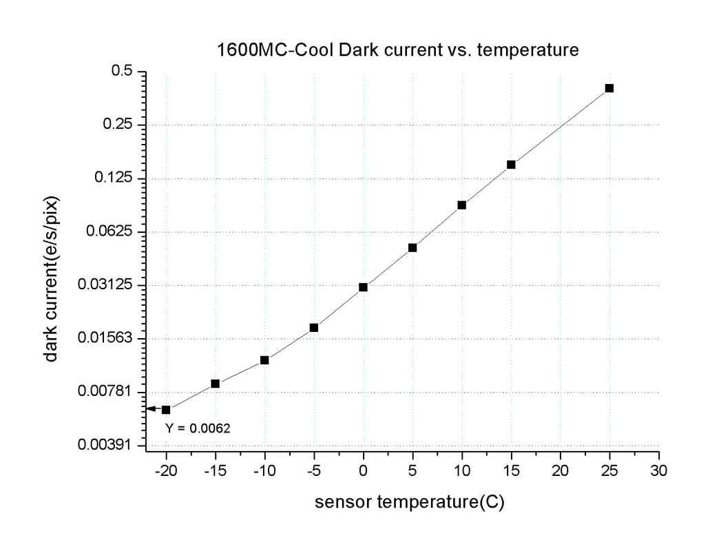 FIGURE 4 - The dark current graph for the popular ZWO ASI 1600mm CMOS sensor.
Dark Current Noise
Another form of noise that can attack an image occurs with changes in temperature. Regarded commonly as thermal noise and more formally as dark current noise, pixels can acquire excess charges when silicon is working at higher temperatures. It is mistakenly thought of a electronics noise, but instead should be thought of a chemical aspect of silicon itself. This is because "photonic" light is not the only thing that can make silicon release an electron.
As a sensor heats up, silicon can be triggered to release an electron that does NOT represent a photon. A typical graph of this noise typically looks like FIGURE 4, which shows a somewhat exponential increase as temperature rises. To put the levels in perspective,
So you are not confused, we are not talking about dark current "signal." Instead, we are talking about what remains AFTER you've done proper dark frame calibration...and it is this
TOWARD A BETTER UNDERSTANDING OF NOISE...
Much of our ideas about noise centers upon the "pixel." In fact, I am convinced that 95% of everybody in this hobby believes that the only reason noise exists in our images is because we use cameras with pixels, with all of their signal-noise ratios (SNR) and noise levels. Obviously, I am not so convinced.
So, first, I think we need to debunk this by realizing that noise will exist regardless of the recording medium, pixel size, or chip technology.
As such, let's pretend that our cameras are "perfect." The ideal camera in that regard would certainly help us with our fight against noise, right?
To me, such a camera would use a technology that records photons precisely where they fall, without arbitrary pixel divisions, using a technology that does not contribute camera noise to an image. If such a camera existed, there would be no perception of pixel divisions, no need for calibration frames - no darks, biases, and flats (except for optical aberrations) - and no electronic noise as a result of read-out electronics and amplification. There's no need to match a camera with a telescope for that perfect "image scale," assuring that the device records at the maximum resolution of the optics themselves.
There would only be object signal and the forces that contribute against it, namely the unavoidable, natural photon noise of the object (more on this later) and the photon noise remnant left over from the already subtracted background light pollution gradient.
So let's do away with pixels and consider the perfect camera. Would it be possible to simulate one? Can we achieve a result that's just as good as this using existing technology. Can we show that noise that comes from the camera doesn't have to be an issue in the final image?
I think we can, indeed!
THE PROBLEM WITH PIXELS...
If I take an image of an object, but do so with a theoretical ZERO pixel camera, then what would be the SNR of the image?
Okay, so this was a trick question.
What would a "zero" pixel camera look like? That's a ridiculous notion...everybody knows that a camera has pixels...and anything that didn't would have to be a film camera...and we know that film is dead.
But wait a second. What was film anyway?
Film was an emulsion of light sensitive particles or "grains" that recorded light where a photon hit. The size of those grains were generally larger than today's pixels, but they were essentially amorphous (differing sizes and shapes). But what if Kodak had made a type of film with almost infinitely small particles? Would this not work as a "zero-pixel" camera?
Or instead, let's pretend that when a photon strikes the camera, it leaves a mark of ink precisely where it hit on the chip. As each ink droplet piles upon another ink droplet, then those areas would begin to saturate...and in the end, you are left with a perfect representation of, perhaps a galaxy, without pixelation. You get the feeling that if you could only magnify the image infinitely, you might be able to see the individual photons themselves?
You see, a camera with ZERO (or infinitely small) pixels isn't so hard to contemplate!
Now ask yourself what noise would look like on such a camera? With film, we used to say that noise would make the image appear "grainy." With digital, we typically say that noise looks "salt and peppery." But how about with the zero pixel camera. Would you perceive noise at all?
The answer to that question is, "Yes. Most certainly!"
In essence, this is what pixels do...because of their size and shape, they give us the opportunity to detect variances between pixel values, and it's this variance BETWEEN pixels which we could perceive as noise within an image.
But this is a deception. In truth, even with the smallest of pixel sizes, we do not need to zoom in to detect noise at the pixel level. In fact, I would argue that doing so is fruitless. "SIDEBAR: Why is Noise So Annoying" talks a little bit more about how noise is perceived within an image, but the short answer is simply to say that noise is usually perceived at larger scales than at the pixel-level. Actually, it typically exists within MULTIPLE larger scales (witness how PixInsight handles noise reduction processes).
The truth is that noise (and SNR on the whole) can only be detected when comparing areas of an image spatially, no matter how large and numerous those areas are. And those things we find objectionable from a noise standpoint are not occurring at the pixel level.
This is contrary to popular digital imaging doctrine that would have you believe that noise needs to be perceived at the pixel-level, with the thought that "what's good for the pixel is what's good for the image." This is a notion that I find faulty.
My argument is that our objection with noise is the result of pixel groups, where pixels of similar noise levels cluster close to each others, forming amorphous blotches within an image. Consequently, I would argue that "pixel peepers" - a term for those who value such individual pixel data - are just wasting their time. In fact, SNR cannot be detected at the pixel level either (see SIDEBAR: Computing SNR for more).
I hear you asking, "But what about hot-pixels and other outlier forms of noise that make the image look terrible?"
Yes, that stuff exists, and we will not overlook such items that can affect an image.
But I would ask you to remember the premise of this article, which is to show you that most noise sources have a very minor contribution to an image, if you are doing it correctly! Where, in fact, our camera is much more PERFECT than you once thought.
Sidebar: Computing SNRWhen imaging the night sky, signal-noise ratio or SNR is not a simple matter of dividing the signal with the noise. Well, it kinda is. The problem is that computing signal is not straight-forward. Neither is calculating noise.
For signal, there is no way of knowing how much light SHOULD be in a single pixel. The best one can do is to take a sampling of MANY similar pixels around a given pixel, compute the average pixel value (mean), and use that value to compute noise, and thus your SNR computation. The larger the neighborhood around a given pixel that is computed, the more accurate the computation will be, unless you start pulling in diversely different pixels from other dissimilar areas. In math speak, we want to sample a sizable number of pixels around a given area of similar features. A "high" SNR will show itself with low standard deviation of values, which can be seen in Photoshop using the Histogram and cursor (see below). 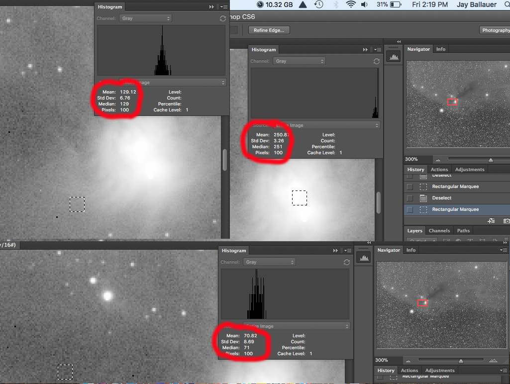
A single frame, uniformly stretched image showing three 10x10 pixel areas of high, medium, and low brightness areas. You can gain an idea of SNR in Photoshop by judging the standard deviation among pixel groups of similar brightness levels. Even then, it's not an accurate, scientific measure (witness the peaked pixels in the highlight histogram), but as long as the sample shows a normal distribution curve on the histogram, you can rely upon it to compare values. Here, it's for illustration only.
In the illustration, the mean pixel value is analogous to the signal level - ignore the fact that the image has been prestretched - of each sampling. This is the average pixel value of all 100 pixels on a scale to 256 in Photoshop (for an ADU approximation, multiply this value by the camera's bit rate minus 8). However, the most accurate way to measure noise level is by computing how those pixels vary from one another, which Photoshop shows as the standard deviation from that mean value. To compute standard deviation, each pixel value is subtracted from the mean value, squared, and averaged together. This number represents the "variance" of the data (or sigma^2). Finally, the square root of the variance is taken to produce the standard deviation (or sigma) for that sampling. Therefore, SNR or signal-noise ratio is calculated as...the ratio of the mean pixel value to the standard deviation of the pixel values over a given neighborhood. In the above illustration, the SNR for the high, medium, and low brightness regions would be 77, 19 and 8 respectively. Interestingly, the pixels themselves are somewhat arbitrary as long as the sample size for that area of the sky is sufficient (you don't want to judge SNR on a only a few pixels). And in truth, there really isn't a need to measure SNR objectively. SNR is more of a subjective thought, typically worded in statements like, "Have I imaged long enough to have a smooth background when I process the image?" Pixel "peepers" will often try to use "pixel SNR" measures to judge performance of an imaging system. But doing so means very little since the eye cannot even detect single pixels (it's not a meaningful, visual measure of image quality) and it typically ignores object signal or overall photon flux of the sampled area. Ironically, as shown, single pixel SNRs can only be computed in the neighborhood with other pixels, which is exactly how the eye evaluates noise in the first place. Likewise, there is no guarantee that the area of sampling comprises equally dispersed photons...larger samples are needed for increased SNR accuracy, yet such samples sizes cover areas of wider signal variance. In such cases, if the sampling of pixels between two different scopes represents the same angular coverage of the night sky, then you should expect similar SNR as long as both scopes have the same aperture, regardless of things such as pixel size, focal length, or f-ratio. See the article called, "The Focal Ratio Myth," for more on this interesting argument. |
I need to add nothing to what Suresh said. But I will say that that thermal noise is predictable, able to be modeled out of the image through dark frame calibration. This is not as evident with DSLRs, that cannot accurately control the camera's operating temperature (hence the reason many, me included, do not take dark frames with DSLRs). However, it's a huge advantage with thermal-electrically cooled astro CCDs. Apply the dark frame and POOF, the thermal noise drops out, and obviously so. Read noise and shot noise are random. They cannot be modeled. However, the noise contribution of camera read noise, as Suresh said, can be made insignificant if your sub-exposure is long enough, where shot noise from the background light swamps out the read noise. Thus, when you image as the "sky-limit" in this way, you come closer to the ideal camera, one without read noise. So, taking as many "sky-limited" sub-exposures as possible is your best way to increase SNR...where it becomes truly the square root of the signal...where this shot noise is the only significant noise source left in the image. Keep in mind that noise sources add quadratically. For example, if your camera has 10 e- of read noise and the background sky glow reaches 1000 e- counts (producing the square root of this as background noise), then you would have sqrt (10^2 + 100^2), or 33.2 total noise...whereas only 1.5 would represent the read noise contribution. So, if you image sufficiently long enough, read noise is not a concern. It varies, but some people use a 5% read noise contribute as the "sky-limit," meaning at this point you have diminishing returns by going longer with the sub-exposure. You might as well just start another exposures, so that you can get the benefits of better outlier rejection when stacking. In above scenario, shot noise would be right at 5% total contribution. So, on a given night with that camera, I would take images AT LEAST as long as where I get the background counts to 1000 ADU. More is okay...less is bring camera read noise more into the picture. ADU = analog to digital units. When you take an image and you see the "screen stretch" in whatever acquisition software you have, the background ADU will be the number that is defined at the left of the histogram curve. One last thing...the background "glow" is actually "signal"...unwanted signal which you remove with the gradient process and then "zero out" with Levels. However, the square root of that LP signal remains in your image as noise (which competes against your object signal). So, ideally, you would want DARK skies, limiting that source of noise. Of course this means that under dark skies you will have to image LONGER with the sub-exposures to achieve "sky-limit." This is why Suresh made the strong comment when he posted his awesome M31 image about the importance of dark skies. Ideally, you want ALL noise contributions to come from OBJECT noise alone. Of course this is not achievable, but you want to climb that asymptote as high as you can. 
|